Indicator Improvement- Part 2- Dealing with Imbalanced Classes
In the previous post, I tried to improve on the outcome of an indicator to distinguish a trend in price changes. It is shown that we can alter time series data and define a classification problem. However, due to the class imbalance, the classification models I used failed. In this post, I’m going to talk about some possible ways to deal with class imbalance.
import matplotlib.pyplot as plt
import numpy as np
import pandas as pd
from sklearn.compose import ColumnTransformer, make_column_transformer
from sklearn.dummy import DummyClassifier
from sklearn.ensemble import RandomForestClassifier
from sklearn.impute import SimpleImputer
from sklearn.linear_model import LogisticRegression
from sklearn.model_selection import (
    TimeSeriesSplit,
    cross_val_score,
    cross_validate,
    train_test_split,
)
from sklearn.pipeline import Pipeline, make_pipeline
from sklearn.preprocessing import OneHotEncoder, OrdinalEncoder, StandardScaler

plt.rcParams["font.size"] = 16
from datetime import datetime
The final data frame that I used for supervised classification methods:
ctgorized_df.head()
| open | high | low | close | open_lag1 | high_lag1 | low_lag1 | close_lag1 | open_lag2 | high_lag2 | ... | high_lag6 | low_lag6 | close_lag6 | sma20 | sma50 | sma100 | trade_hour | dis_to_max_12bar | dis_to_min_12bar | market-type | |
|---|---|---|---|---|---|---|---|---|---|---|---|---|---|---|---|---|---|---|---|---|---|
| 0 | 0.87138 | 0.87138 | 0.87064 | 0.87103 | 0.87093 | 0.87156 | 0.87056 | 0.87139 | 0.87088 | 0.87134 | ... | 0.87217 | 0.87121 | 0.87161 | 0.871588 | 0.871522 | 0.872727 | 10.0 | 0.00291 | 0.00015 | UpTrend-PriceDown |
| 1 | 0.86942 | 0.87013 | 0.86900 | 0.87012 | 0.86939 | 0.86976 | 0.86913 | 0.86943 | 0.86988 | 0.87028 | ... | 0.87070 | 0.87012 | 0.87050 | 0.871093 | 0.871101 | 0.872387 | 10.0 | 0.00127 | 0.00076 | DownTrend-PriceUp |
| 2 | 0.86411 | 0.86417 | 0.86403 | 0.86409 | 0.86409 | 0.86416 | 0.86407 | 0.86409 | 0.86395 | 0.86412 | ... | 0.86400 | 0.86353 | 0.86389 | 0.863412 | 0.863401 | 0.864325 | 22.0 | 0.00042 | 0.00121 | UpTrend-NoTrend |
| 3 | 0.86455 | 0.86470 | 0.86453 | 0.86469 | 0.86441 | 0.86456 | 0.86422 | 0.86456 | 0.86467 | 0.86468 | ... | 0.86483 | 0.86466 | 0.86471 | 0.864797 | 0.864814 | 0.864159 | 2.0 | 0.00019 | 0.00028 | DownTrend-NoTrend |
| 4 | 0.86504 | 0.86504 | 0.86430 | 0.86468 | 0.86527 | 0.86536 | 0.86500 | 0.86502 | 0.86504 | 0.86530 | ... | 0.86484 | 0.86461 | 0.86479 | 0.864798 | 0.864798 | 0.864729 | 6.0 | 0.00065 | 0.00015 | UpTrend_PriceUp |
5 rows × 35 columns
ctgorized_df['market-type'].value_counts()
DownTrend-NoTrend      2255
UpTrend-NoTrend        2237
UpTrend_PriceUp         238
DownTrend-PriceUp       228
UpTrend-PriceDown       218
DownTrend-PriceDown     208
Name: market-type, dtype: int64
There are several methods to deal with imbalanced classes in machine learning classifications. Some of them define different cost functions proportional to class populations, which is called cost-sensitive learning. Another category of methods deals with the way we are doing sampling. In simple words, take more samples from low-population classes or fewer samples from more-populated classes. Of course, the way they do this is more complicated than what I explained here. I’m going to use one of these sampling methods here and compare their outcomes with what I have found in my previous blog post. If you are interested to learn more about the sampling methods, take a look at this blog post.
Using the sampling methods to balance the classes has drawbacks! You either remove information or cause overfitting of the model. However, sometimes the nature of your data might help you to decrease the imbalanced classes issue! If you read the previous post, I mentioned that indeed the forex market is a 24-hour market, but it does not mean that it is always active! Let me show you the standard deviation of the price differences between the close price and its maximum/minimum during 12 data points (one hour) for 24 hours of the day!
diff_to_max = ctgorized_df.groupby('trade_hour')['dis_to_max_12bar'].std()
diff_to_mis = ctgorized_df.groupby('trade_hour')['dis_to_min_12bar'].std()
volatility = diff_to_max + diff_to_mis
plt.figure()
plt.rcParams["figure.figsize"] = (10,7)
plt.bar(volatility.index, volatility)
plt.axhline(y=0.0010, color='r', linestyle='-')
plt.show()
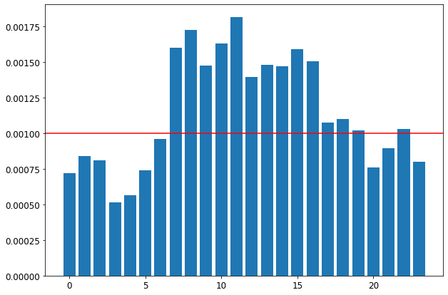
As can be seen, the summation of the standard deviations of the price differences from maximum and minimum during some hours of the day is less than 10 pips (0.0010)! So, the probability of having a price change of more than 10 pips during those hours is low!
One thing I should emphasize here is that I do not do classification for the classification! I’m looking for profitable trades! I do not have to trade during those hours if the market is not volatile enough! Let’s remove those hours from the data and see the total numbers of each class.
ctgorized_sub_df = ctgorized_df[(ctgorized_df['trade_hour']>= 7) & (ctgorized_df['trade_hour']<= 19)]
ctgorized_sub_df['market-type'].value_counts()
DownTrend-NoTrend      993
UpTrend-NoTrend        974
UpTrend_PriceUp        200
DownTrend-PriceUp      173
UpTrend-PriceDown      166
DownTrend-PriceDown    163
Name: market-type, dtype: int64
That is much better! So, now let’s see how the classification methods work. As always, split data to the train and test data frame, and fit our models.
train-test split
train_df, test_df = train_test_split(ctgorized_sub_df, test_size=0.2, random_state=42)
train_df['market-type'].value_counts()
DownTrend-NoTrend      813
UpTrend-NoTrend        766
UpTrend_PriceUp        159
UpTrend-PriceDown      138
DownTrend-PriceDown    130
DownTrend-PriceUp      129
Name: market-type, dtype: int64
test_df['market-type'].value_counts()
UpTrend-NoTrend        208
DownTrend-NoTrend      180
DownTrend-PriceUp       44
UpTrend_PriceUp         41
DownTrend-PriceDown     33
UpTrend-PriceDown       28
Name: market-type, dtype: int64
Preprocessing the data
train_df.columns
Index(['open', 'high', 'low', 'close', 'open_lag1', 'high_lag1', 'low_lag1',
       'close_lag1', 'open_lag2', 'high_lag2', 'low_lag2', 'close_lag2',
       'open_lag3', 'high_lag3', 'low_lag3', 'close_lag3', 'open_lag4',
       'high_lag4', 'low_lag4', 'close_lag4', 'open_lag5', 'high_lag5',
       'low_lag5', 'close_lag5', 'open_lag6', 'high_lag6', 'low_lag6',
       'close_lag6', 'sma20', 'sma50', 'sma100', 'trade_hour',
       'dis_to_max_12bar', 'dis_to_min_12bar', 'market-type'],
      dtype='object')
numeric_features = ['open', 'high', 'low', 'close', 'open_lag1', 'high_lag1', 'low_lag1',
       'close_lag1', 'open_lag2', 'high_lag2', 'low_lag2', 'close_lag2',
       'open_lag3', 'high_lag3', 'low_lag3', 'close_lag3', 'open_lag4',
       'high_lag4', 'low_lag4', 'close_lag4', 'open_lag5', 'high_lag5',
       'low_lag5', 'close_lag5', 'open_lag6', 'high_lag6', 'low_lag6',
       'close_lag6', 'sma20', 'sma50', 'sma100',
       'dis_to_max_12bar', 'dis_to_min_12bar', ]

ordinal_features = ['trade_hour']

drop_features = ['market-type']
numeric_transform = make_pipeline(StandardScaler())

preprocessor = make_column_transformer(
    (numeric_transform, numeric_features),
    ('passthrough', ordinal_features),
    ('drop', drop_features)
)

preprocessor.fit(train_df)

new_clomuns = numeric_features + ordinal_features
X_train  = pd.DataFrame(preprocessor.transform(train_df), index=train_df.index, columns=new_clomuns)
X_test  = pd.DataFrame(preprocessor.transform(test_df), index=test_df.index, columns=new_clomuns)

y_train = train_df['market-type']
y_test = test_df['market-type']

print(X_train.shape, X_test.shape, y_train.shape, y_test.shape)
(2135, 34) (534, 34) (2135,) (534,)
Classification
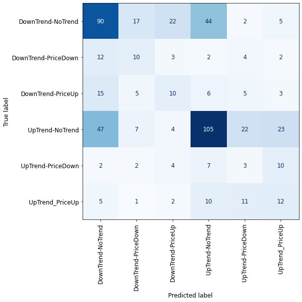
I only use the Random Over Sampling method for dealing with imbalanced classes. After producing a proper training data frame with this method, do the classification with the Random Forest and the Support Vector Machine supervised learning models from the sklearn library.
#confusion matrix
from sklearn.metrics import ConfusionMatrixDisplay
def plot_confusion_matrix_classifier(clf):
    plt.rc('font', size=12)
    disp = ConfusionMatrixDisplay.from_estimator(
        clf,
        X_test,
        y_test,
        display_labels=dummy.classes_,
        values_format="d",
        cmap=plt.cm.Blues,
        colorbar=False,
    )

    plt.xticks(rotation = 90)
    fig = disp.ax_.get_figure()
    fig.set_figwidth(8)
    fig.set_figheight(8)
Random over sampling
# import library
from imblearn.over_sampling import RandomOverSampler

ros = RandomOverSampler(random_state=123)
X_train_ros, y_train_ros = ros.fit_resample(X_train, y_train)
from sklearn.ensemble import RandomForestClassifier
rfc = RandomForestClassifier(max_depth=10, random_state=0)
rfc.fit(X_train_ros, y_train_ros)
plot_confusion_matrix_classifier(rfc)   #plotting the confusion matrix for X_test and y_test
from sklearn.svm import SVC
svc = SVC(kernel='rbf', probability=True)
svc.fit(X_train_ros, y_train_ros)
plot_confusion_matrix_classifier(svc)   #plotting the confusion matrix for X_test and y_test
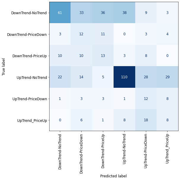
In comparison with the previous outcomes of our supervised learning models, after balancing the classes, we have a significant improvement in our models. However, classification-wise, the results are not acceptable yet! One big reason goes back to the nature of the market fluctuations which can suddenly change their direction. This effect is less significant for the larger time frames. Also, if you are interested, you can try this methodology for other trend indicators, that might provide better outcomes.