Indicator Improvement- Part 1- A supervised classification learning
As a trader, I do not need to predict the final price to be able to make a profit! As far as I could distinguish a trend in the price change, I can enter a trade and make a profit. This is the mindset of the majority of the scalpers and the day traders! Over a years, lots of methods and trading strategies have been developed for this aim. In the trading world, people are looking to the indicators to get trading pulses! For example, when a 20-bar simple moving average (SMA) passes and goes above the 50-bar SMA, that indicates an up trend in the price, so people get a long trade. Unfortunately, these indicators do not work well, and the nature of the market can be much more complicated. Here, I want to see if a supervised ML algorithm can help us to improve this indicator!
What I am going to do here is not a regression, but classification! I need to know whether the indicator can show the up or down trends or not! Therefore, I need to alter the time series data frame to satisfy this purpose. Let’s start with importing libraries and data.
import matplotlib.pyplot as plt
import numpy as np
import pandas as pd
from sklearn.compose import ColumnTransformer, make_column_transformer
from sklearn.dummy import DummyClassifier
from sklearn.ensemble import RandomForestClassifier
from sklearn.impute import SimpleImputer
from sklearn.linear_model import LogisticRegression
from sklearn.model_selection import (
    TimeSeriesSplit,
    cross_val_score,
    cross_validate,
    train_test_split,
)
from sklearn.pipeline import Pipeline, make_pipeline
from sklearn.preprocessing import OneHotEncoder, OrdinalEncoder, StandardScaler

plt.rcParams["font.size"] = 16
from datetime import datetime
from google.colab import drive
drive.mount('/content/gdrive')
Drive already mounted at /content/gdrive; to attempt to forcibly remount, call drive.mount("/content/gdrive", force_remount=True).
fx_df = pd.read_csv('/content/gdrive/MyDrive/Python-Colab-Projects/Forex_Data/EURGBP_Candlestick_5_M_BID_14.10.2019-14.10.2022.csv')
fx_df.head()
| Gmt time | Open | High | Low | Close | Volume | |
|---|---|---|---|---|---|---|
| 0 | 15.10.2019 00:00:00.000 | 0.87438 | 0.87461 | 0.87429 | 0.87430 | 434.60 |
| 1 | 15.10.2019 00:05:00.000 | 0.87430 | 0.87440 | 0.87418 | 0.87440 | 402.75 |
| 2 | 15.10.2019 00:10:00.000 | 0.87441 | 0.87450 | 0.87439 | 0.87448 | 421.10 |
| 3 | 15.10.2019 00:15:00.000 | 0.87448 | 0.87451 | 0.87436 | 0.87441 | 342.43 |
| 4 | 15.10.2019 00:20:00.000 | 0.87441 | 0.87444 | 0.87435 | 0.87443 | 195.58 |
When the market is closed, the prices are set on the last price of the active market. However, I can find those times by looking at the volume of the trades and dropping them.
fx_df.loc[fx_df['Volume'] == 0].head()
| Gmt time | Open | High | Low | Close | Volume | |
|---|---|---|---|---|---|---|
| 1116 | 18.10.2019 21:00:00.000 | 0.86047 | 0.86047 | 0.86047 | 0.86047 | 0.0 |
| 1117 | 18.10.2019 21:05:00.000 | 0.86047 | 0.86047 | 0.86047 | 0.86047 | 0.0 |
| 1118 | 18.10.2019 21:10:00.000 | 0.86047 | 0.86047 | 0.86047 | 0.86047 | 0.0 |
| 1119 | 18.10.2019 21:15:00.000 | 0.86047 | 0.86047 | 0.86047 | 0.86047 | 0.0 |
| 1120 | 18.10.2019 21:20:00.000 | 0.86047 | 0.86047 | 0.86047 | 0.86047 | 0.0 |
fx_df_active = fx_df.loc[fx_df['Volume'] != 0]
fx_df_active.loc[fx_df_active['Volume'] == 0].any()
Gmt time    False
Open        False
High        False
Low         False
Close       False
Volume      False
dtype: bool
Checking for missing data:
fx_df_active.isnull().any()
Gmt time    False
Open        False
High        False
Low         False
Close       False
Volume      False
dtype: bool
Now, convert the index to the date-time. Also, I want to remove the volume column and go just with the time and price analysis.
fx_df_active.columns = ['date', 'open', 'high', 'low', 'close', 'volume']
fx_df_active.loc[:, 'date'] = pd.to_datetime(fx_df_active.loc[:, 'date'] , format='%d.%m.%Y %H:%M:%S.%f')
fx_df_active = fx_df_active.set_index(fx_df_active.loc[:, 'date'])
fx_df_5m = fx_df_active[['open', 'high', 'low', 'close', 'volume']]
fx_df_5m = fx_df_5m.drop_duplicates(keep=False)
/usr/local/lib/python3.7/dist-packages/pandas/core/indexing.py:1773: SettingWithCopyWarning:
A value is trying to be set on a copy of a slice from a DataFrame.
Try using .loc[row_indexer,col_indexer] = value instead

See the caveats in the documentation: https://pandas.pydata.org/pandas-docs/stable/user_guide/indexing.html#returning-a-view-versus-a-copy
  self._setitem_single_column(ilocs[0], value, pi)
fx_df_5m_prices = fx_df_5m.drop(['volume'], axis=1) #dropping volume column
fx_df_5m_prices.head()
| open | high | low | close | |
|---|---|---|---|---|
| date | ||||
| 2019-10-15 00:00:00 | 0.87438 | 0.87461 | 0.87429 | 0.87430 |
| 2019-10-15 00:05:00 | 0.87430 | 0.87440 | 0.87418 | 0.87440 |
| 2019-10-15 00:10:00 | 0.87441 | 0.87450 | 0.87439 | 0.87448 |
| 2019-10-15 00:15:00 | 0.87448 | 0.87451 | 0.87436 | 0.87441 |
| 2019-10-15 00:20:00 | 0.87441 | 0.87444 | 0.87435 | 0.87443 |
Similar to the previous work, I am adding the lagged data and the simple moving averages to the data frame.
fx_lag_prices_df = fx_df_5m_prices.copy()
for i in range(1,7):
    forex_data_lag = fx_df_5m_prices.shift(i)
    lag_columns = list( s+"_lag%d" % i for s in fx_df_5m_prices.columns)
    forex_data_lag.columns = lag_columns
    fx_lag_prices_df = pd.concat([fx_lag_prices_df, forex_data_lag], axis =1)
def simple_moving_average(data, moving_average_list, criteria='close'):
    df = pd.DataFrame()
    for ma in moving_average_list:
        sma_column = f"sma{ma}"
        sma = data[criteria].rolling(center=False, window = ma).mean().to_frame(name = sma_column)
        df = pd.concat((df, sma),  axis=1)

    return(df )

sma_df = simple_moving_average(fx_df_5m_prices, [20, 50, 100])
fx_lag_prices_sma_df = pd.concat([fx_lag_prices_df, sma_df], axis =1)
fx_lag_prices_sma_df.head()
| open | high | low | close | open_lag1 | high_lag1 | low_lag1 | close_lag1 | open_lag2 | high_lag2 | ... | high_lag5 | low_lag5 | close_lag5 | open_lag6 | high_lag6 | low_lag6 | close_lag6 | sma20 | sma50 | sma100 | |
|---|---|---|---|---|---|---|---|---|---|---|---|---|---|---|---|---|---|---|---|---|---|
| date | |||||||||||||||||||||
| 2019-10-15 00:00:00 | 0.87438 | 0.87461 | 0.87429 | 0.87430 | NaN | NaN | NaN | NaN | NaN | NaN | ... | NaN | NaN | NaN | NaN | NaN | NaN | NaN | NaN | NaN | NaN |
| 2019-10-15 00:05:00 | 0.87430 | 0.87440 | 0.87418 | 0.87440 | 0.87438 | 0.87461 | 0.87429 | 0.87430 | NaN | NaN | ... | NaN | NaN | NaN | NaN | NaN | NaN | NaN | NaN | NaN | NaN |
| 2019-10-15 00:10:00 | 0.87441 | 0.87450 | 0.87439 | 0.87448 | 0.87430 | 0.87440 | 0.87418 | 0.87440 | 0.87438 | 0.87461 | ... | NaN | NaN | NaN | NaN | NaN | NaN | NaN | NaN | NaN | NaN |
| 2019-10-15 00:15:00 | 0.87448 | 0.87451 | 0.87436 | 0.87441 | 0.87441 | 0.87450 | 0.87439 | 0.87448 | 0.87430 | 0.87440 | ... | NaN | NaN | NaN | NaN | NaN | NaN | NaN | NaN | NaN | NaN |
| 2019-10-15 00:20:00 | 0.87441 | 0.87444 | 0.87435 | 0.87443 | 0.87448 | 0.87451 | 0.87436 | 0.87441 | 0.87441 | 0.87450 | ... | NaN | NaN | NaN | NaN | NaN | NaN | NaN | NaN | NaN | NaN |
5 rows × 31 columns
The forex market is indeed a 24-hour market, but it does not mean that it is always active! The active hours of the forex market are in tune with the active hours of other markets in Europe and the USA. So, it is good the add the trading hours as a feature to our data frame.
fx_df_5m.index.hour.unique().values
array([ 0,  1,  2,  3,  4,  5,  6,  7,  8,  9, 10, 11, 12, 13, 14, 15, 16,
       17, 18, 19, 20, 21, 22, 23])
fx_lag_prices_sma_hour_df = fx_lag_prices_sma_df.copy()
fx_lag_prices_sma_hour_df['trade_hour'] = fx_lag_prices_sma_hour_df.index.hour
Another feature I am going to add to the data frame is the differences between the current closing price with the maximum/minimum of the price in the past data points. Each data point (bar, as it is called) in our 5-min chart shows opening and closing prices as well as the maximum and minimum of the price in a 5-minute interval.
fx_lag_prices_sma_hour_minmax_df = fx_lag_prices_sma_hour_df.copy()
n_minmax = 12  #number of the past data points
clmn_min = f'dis_to_min_{n_minmax}bar'
clmn_max = f'dis_to_max_{n_minmax}bar'
fx_lag_prices_sma_hour_minmax_df[clmn_max] = 0
fx_lag_prices_sma_hour_minmax_df[clmn_min] = 0
for i in range(0,len(fx_lag_prices_sma_hour_df)):
    if i < n_minmax:
       dis_to_max = fx_lag_prices_sma_hour_minmax_df['close'].iloc[0:i+1].max() - fx_lag_prices_sma_hour_minmax_df['close'].iloc[i]
       fx_lag_prices_sma_hour_minmax_df[clmn_max].iloc[i] = dis_to_max

       dis_to_min = fx_lag_prices_sma_hour_minmax_df['close'].iloc[i] - fx_lag_prices_sma_hour_minmax_df['close'].iloc[0:i+1].min()
       fx_lag_prices_sma_hour_minmax_df[clmn_min].iloc[i] = dis_to_min

    else:
       dis_to_max = fx_lag_prices_sma_hour_minmax_df['close'].iloc[i-n_minmax:i+1].max() - fx_lag_prices_sma_hour_minmax_df['close'].iloc[i]
       fx_lag_prices_sma_hour_minmax_df[clmn_max].iloc[i] = dis_to_max

       dis_to_min = fx_lag_prices_sma_hour_minmax_df['close'].iloc[i] - fx_lag_prices_sma_hour_minmax_df['close'].iloc[i-n_minmax:i+1].min()
       fx_lag_prices_sma_hour_minmax_df[clmn_min].iloc[i] = dis_to_min
Usually, I copied the last feature-engineered data frame, to a new one. In this way, by changing the features, it is easier to update the rest of the program and models.
exd_df_final = fx_lag_prices_sma_hour_minmax_df.dropna()
exd_df_final.head()
| open | high | low | close | open_lag1 | high_lag1 | low_lag1 | close_lag1 | open_lag2 | high_lag2 | ... | open_lag6 | high_lag6 | low_lag6 | close_lag6 | sma20 | sma50 | sma100 | trade_hour | dis_to_max_12bar | dis_to_min_12bar | |
|---|---|---|---|---|---|---|---|---|---|---|---|---|---|---|---|---|---|---|---|---|---|
| date | |||||||||||||||||||||
| 2019-10-15 08:15:00 | 0.87099 | 0.87114 | 0.87055 | 0.87104 | 0.87096 | 0.87122 | 0.87073 | 0.87098 | 0.87068 | 0.87165 | ... | 0.87022 | 0.87082 | 0.87017 | 0.87048 | 0.871091 | 0.872396 | 0.873362 | 8 | 0.00052 | 0.00099 |
| 2019-10-15 08:20:00 | 0.87107 | 0.87187 | 0.87092 | 0.87179 | 0.87099 | 0.87114 | 0.87055 | 0.87104 | 0.87096 | 0.87122 | ... | 0.87048 | 0.87127 | 0.87027 | 0.87091 | 0.871109 | 0.872345 | 0.873337 | 8 | 0.00000 | 0.00174 |
| 2019-10-15 08:25:00 | 0.87179 | 0.87179 | 0.87044 | 0.87080 | 0.87107 | 0.87187 | 0.87092 | 0.87179 | 0.87099 | 0.87114 | ... | 0.87091 | 0.87156 | 0.87080 | 0.87156 | 0.871094 | 0.872275 | 0.873301 | 8 | 0.00099 | 0.00075 |
| 2019-10-15 08:30:00 | 0.87080 | 0.87116 | 0.87013 | 0.87045 | 0.87179 | 0.87179 | 0.87044 | 0.87080 | 0.87107 | 0.87187 | ... | 0.87155 | 0.87161 | 0.87056 | 0.87069 | 0.871031 | 0.872200 | 0.873260 | 8 | 0.00134 | 0.00024 |
| 2019-10-15 08:35:00 | 0.87045 | 0.87062 | 0.87008 | 0.87062 | 0.87080 | 0.87116 | 0.87013 | 0.87045 | 0.87179 | 0.87179 | ... | 0.87068 | 0.87165 | 0.87054 | 0.87097 | 0.870946 | 0.872130 | 0.873223 | 8 | 0.00117 | 0.00041 |
5 rows × 34 columns
Now, the most important part is: what is the target?
As I explained at the beginning, I expect an up trend if 20-bar SMA goes above 50-bar SMA, and a downtrend if it goes in the opposite way. But, the reality might be different from my expectation. So, let’s look at the behavior of the close price, during 10 data points after 20-bar SMA passes the 50-Bar SMA.
So, the new data frame only includes the data of the passing points. The target is the behavior of the close price and its difference from our expectations. For example, if we expect an up trend, but in the next 10 data points, the minimum price moves downwards by 0.0010 (10 pips), I classified this data point as “UpTrend-PriceDown”. Here, the first part (UpTrend) shows my expectation from the indicator, and the second part (PriceDown) shows the actual behavior of the price in 10 data points in the future. Other defined classes are distinguished in the comments.
pred_windo = 10
pip_val = 0.0010 #10 pips
df_size = len(exd_df_final)

ctgorized_df_columns = list(list(exd_df_final.columns) +  ['market-type'] )
ctgorized_df = pd.DataFrame(columns = ctgorized_df_columns)

_row_series = []
for i in range(1, df_size - pred_windo):
#for i in range(1, 1000):
    if exd_df_final['sma20'][i-1] <= exd_df_final['sma50'][i-1]:
        if exd_df_final['sma20'][i] > exd_df_final['sma50'][i]:  #Expecting a Bull market
            if exd_df_final['close'][i:i+pred_windo].max() - exd_df_final['close'][i] > pip_val:
                if exd_df_final['close'][i] - exd_df_final['close'][i:i+pred_windo].min() < pip_val:
                    mkt = 'UpTrend_PriceUp'  #Expecting an up trend, the price goes up
            if exd_df_final['close'][i:i+pred_windo].max() - exd_df_final['close'][i] < pip_val:
                if exd_df_final['close'][i] - exd_df_final['close'][i:i+pred_windo].min() > pip_val:
                    mkt = 'UpTrend-PriceDown'   #Expecting an up trend, the price goes down
            if exd_df_final['close'][i:i+pred_windo].max() - exd_df_final['close'][i] > pip_val:
                if exd_df_final['close'][i] - exd_df_final['close'][i:i+pred_windo].min() > pip_val:
                    mkt = 'UpTrend-Volatile'    #Expecting an up trend, the price moves in both ways
            if exd_df_final['close'][i:i+pred_windo].max() - exd_df_final['close'][i] < pip_val:
                if exd_df_final['close'][i] - exd_df_final['close'][i:i+pred_windo].min() < pip_val:
                    mkt = 'UpTrend-NoTrend'  #Expecting an up trend, the price does not change by 10 pips

            _row_series = pd.Series(exd_df_final.iloc[i,:])
            _row_series = list(list(_row_series) + [mkt])

            ctgorized_df = ctgorized_df.append(pd.Series(_row_series,
                                                         index = ctgorized_df_columns),
                                               ignore_index = True, sort = False)

    if exd_df_final['sma20'][i-1] >= exd_df_final['sma50'][i-1]:
        if exd_df_final['sma20'][i] < exd_df_final['sma50'][i]: #Expecting a Bear market
            if exd_df_final['close'][i:i+pred_windo].max() - exd_df_final['close'][i] < pip_val:
                if exd_df_final['close'][i] - exd_df_final['close'][i:i+pred_windo].min() > pip_val:
                    mkt = 'DownTrend-PriceDown' #Expecting a down trend, the price goes down
            if exd_df_final['close'][i:i+pred_windo].max() - exd_df_final['close'][i] > pip_val:
                if exd_df_final['close'][i] - exd_df_final['close'][i:i+pred_windo].min() < pip_val:
                    mkt = 'DownTrend-PriceUp'   #Expecting a down trend, the price goes up
            if exd_df_final['close'][i:i+pred_windo].max() - exd_df_final['close'][i] > pip_val:
                if exd_df_final['close'][i] - exd_df_final['close'][i:i+pred_windo].min() > pip_val:
                    mkt = 'DownTrend-Volatile'  #Expecting a down trend, the price moves in both ways
            if exd_df_final['close'][i:i+pred_windo].max() - exd_df_final['close'][i] < pip_val:
                if exd_df_final['close'][i] - exd_df_final['close'][i:i+pred_windo].min() < pip_val:
                    mkt = 'DownTrend-NoTrend'    #Expecting a down trend, the price does not change by 10 pips

            _row_series = pd.Series(exd_df_final.iloc[i,:])
            _row_series = list(list(_row_series) + [mkt])

            ctgorized_df = ctgorized_df.append(pd.Series(_row_series,
                                                         index = ctgorized_df_columns),
                                               ignore_index = True, sort = False)
ctgorized_df.head()
| open | high | low | close | open_lag1 | high_lag1 | low_lag1 | close_lag1 | open_lag2 | high_lag2 | ... | high_lag6 | low_lag6 | close_lag6 | sma20 | sma50 | sma100 | trade_hour | dis_to_max_12bar | dis_to_min_12bar | market-type | |
|---|---|---|---|---|---|---|---|---|---|---|---|---|---|---|---|---|---|---|---|---|---|
| 0 | 0.87138 | 0.87138 | 0.87064 | 0.87103 | 0.87093 | 0.87156 | 0.87056 | 0.87139 | 0.87088 | 0.87134 | ... | 0.87217 | 0.87121 | 0.87161 | 0.871588 | 0.871522 | 0.872727 | 10.0 | 0.00291 | 0.00015 | UpTrend-PriceDown |
| 1 | 0.86942 | 0.87013 | 0.86900 | 0.87012 | 0.86939 | 0.86976 | 0.86913 | 0.86943 | 0.86988 | 0.87028 | ... | 0.87070 | 0.87012 | 0.87050 | 0.871093 | 0.871101 | 0.872387 | 10.0 | 0.00127 | 0.00076 | DownTrend-PriceUp |
| 2 | 0.86411 | 0.86417 | 0.86403 | 0.86409 | 0.86409 | 0.86416 | 0.86407 | 0.86409 | 0.86395 | 0.86412 | ... | 0.86400 | 0.86353 | 0.86389 | 0.863412 | 0.863401 | 0.864325 | 22.0 | 0.00042 | 0.00121 | UpTrend-NoTrend |
| 3 | 0.86455 | 0.86470 | 0.86453 | 0.86469 | 0.86441 | 0.86456 | 0.86422 | 0.86456 | 0.86467 | 0.86468 | ... | 0.86483 | 0.86466 | 0.86471 | 0.864797 | 0.864814 | 0.864159 | 2.0 | 0.00019 | 0.00028 | DownTrend-NoTrend |
| 4 | 0.86504 | 0.86504 | 0.86430 | 0.86468 | 0.86527 | 0.86536 | 0.86500 | 0.86502 | 0.86504 | 0.86530 | ... | 0.86484 | 0.86461 | 0.86479 | 0.864798 | 0.864798 | 0.864729 | 6.0 | 0.00065 | 0.00015 | UpTrend_PriceUp |
5 rows × 35 columns
ctgorized_df['market-type'].value_counts()
DownTrend-NoTrend      2255
UpTrend-NoTrend        2237
UpTrend_PriceUp         238
DownTrend-PriceUp       228
UpTrend-PriceDown       218
DownTrend-PriceDown     208
DownTrend-Volatile       12
UpTrend-Volatile          8
Name: market-type, dtype: int64
As can be seen, the defined classes are very imbalanced. The last two classes rarely happen, so, I’ll start by dropping them. Later, I’ll deal with imbalances in a separate blog post, but for now, let’s see how much a classification ML algorithm is successful to classify this problem.
ctgorized_df.drop(ctgorized_df[ctgorized_df['market-type']=='DownTrend-Volatile'].index, inplace=True)
ctgorized_df.drop(ctgorized_df[ctgorized_df['market-type']=='UpTrend-Volatile'].index, inplace=True)
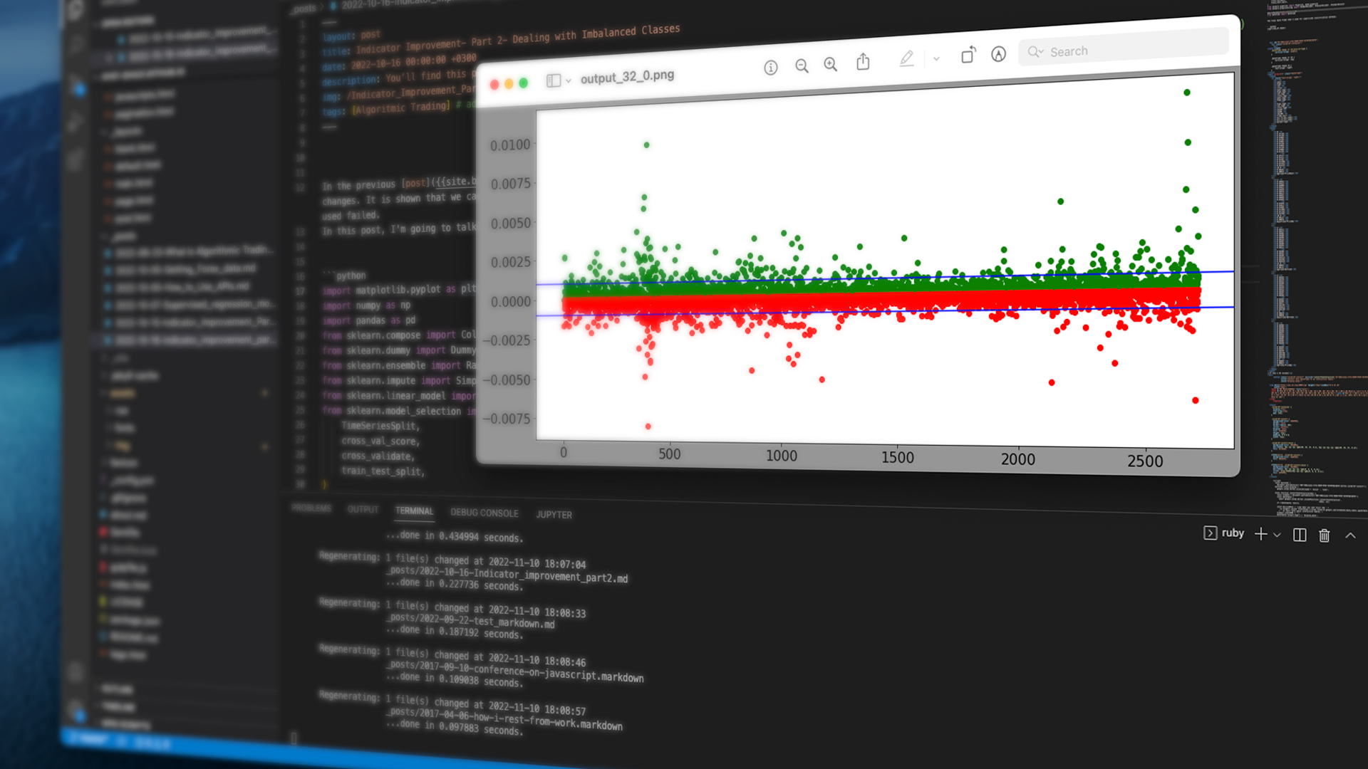
Besides the imbalanced classes, we can understand that the indicator we are looking at, is not a good indicator to show the trend. Let me show the graph of the price changes when we expect to have an up trend!
df_size = len(exd_df_final)

up_up_series = []
up_down_series = []

for i in range(1, df_size - pred_windo):
    if exd_df_final['sma20'][i-1] <= exd_df_final['sma50'][i-1]:
        if exd_df_final['sma20'][i] > exd_df_final['sma50'][i]:  #Bull market
            bull_max_dif = exd_df_final['close'][i:i+pred_windo].max() - exd_df_final['close'][i]
            up_up_series.append(bull_max_dif)
            bull_min_dif = exd_df_final['close'][i] - exd_df_final['close'][i:i+pred_windo].min()
            up_down_series.append(-1*bull_min_dif)
plt.figure()
plt.rcParams["figure.figsize"] = (15,7)
plt.scatter(range(len(up_up_series)),up_up_series, marker='o', c='g')
plt.axhline(y=0.0010, color='b', linestyle='-')
plt.scatter(range(len(up_down_series)),up_down_series, marker='o', c='r')
plt.axhline(y=-0.0010, color='b', linestyle='-')
plt.show()
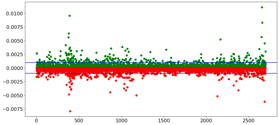
It seems that our indicator cannot identify a trend! the change in the price can be in any direction, and most of the time, the price does not change as much as we expected! You might get better results if started with some indicators that have been developed to identify the trends.
Train-Test split
Now, it is time to prepare our data for a classification learning method. Since I altered the problem to a classification, and do not deal with a time series anymore, I can use the Sklear train-test-split function.
train_df, test_df = train_test_split(ctgorized_df, test_size=0.2, random_state=42)
train_df['market-type'].value_counts()
UpTrend-NoTrend        1806
DownTrend-NoTrend      1797
DownTrend-PriceUp       189
UpTrend_PriceUp         182
UpTrend-PriceDown       179
DownTrend-PriceDown     154
Name: market-type, dtype: int64
test_df['market-type'].value_counts()
DownTrend-NoTrend      458
UpTrend-NoTrend        431
UpTrend_PriceUp         56
DownTrend-PriceDown     54
DownTrend-PriceUp       39
UpTrend-PriceDown       39
Name: market-type, dtype: int64
Preprocessing the data
train_df.columns
Index(['open', 'high', 'low', 'close', 'open_lag1', 'high_lag1', 'low_lag1',
       'close_lag1', 'open_lag2', 'high_lag2', 'low_lag2', 'close_lag2',
       'open_lag3', 'high_lag3', 'low_lag3', 'close_lag3', 'open_lag4',
       'high_lag4', 'low_lag4', 'close_lag4', 'open_lag5', 'high_lag5',
       'low_lag5', 'close_lag5', 'open_lag6', 'high_lag6', 'low_lag6',
       'close_lag6', 'sma20', 'sma50', 'sma100', 'trade_hour',
       'dis_to_max_12bar', 'dis_to_min_12bar', 'market-type'],
      dtype='object')
numeric_features = ['open', 'high', 'low', 'close', 'open_lag1', 'high_lag1', 'low_lag1',
       'close_lag1', 'open_lag2', 'high_lag2', 'low_lag2', 'close_lag2',
       'open_lag3', 'high_lag3', 'low_lag3', 'close_lag3', 'open_lag4',
       'high_lag4', 'low_lag4', 'close_lag4', 'open_lag5', 'high_lag5',
       'low_lag5', 'close_lag5', 'open_lag6', 'high_lag6', 'low_lag6',
       'close_lag6', 'sma20', 'sma50', 'sma100',
       'dis_to_max_12bar', 'dis_to_min_12bar', ]

ordinal_features = ['trade_hour']

drop_features = ['market-type']
numeric_transform = make_pipeline(StandardScaler())

preprocessor = make_column_transformer(
    (numeric_transform, numeric_features),
    ('passthrough', ordinal_features),
    ('drop', drop_features)
)

preprocessor.fit(train_df)

new_clomuns = numeric_features + ordinal_features
X_train  = pd.DataFrame(preprocessor.transform(train_df), index=train_df.index, columns=new_clomuns)
X_test  = pd.DataFrame(preprocessor.transform(test_df), index=test_df.index, columns=new_clomuns)

y_train = train_df['market-type']
y_test = test_df['market-type']

print(X_train.shape, X_test.shape, y_train.shape, y_test.shape)
(4307, 34) (1077, 34) (4307,) (1077,)
Classification
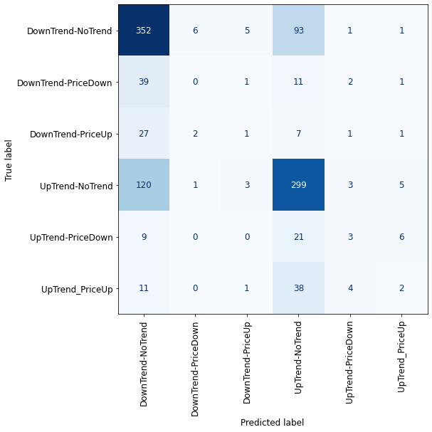
Due to class imbalance, cross-validation is not a good criterion to validate our model. To have a good understanding of how our classes are classified, I use the Confusion matrix.
from sklearn.metrics import ConfusionMatrixDisplay

def plot_confusion_matrix_classifier(clf):
    plt.rc('font', size=12)
    disp = ConfusionMatrixDisplay.from_estimator(
        clf,
        X_test,
        y_test,
        display_labels=dummy.classes_,
        values_format="d",
        cmap=plt.cm.Blues,
        colorbar=False,
    )

    plt.xticks(rotation = 90)
    fig = disp.ax_.get_figure()
    fig.set_figwidth(8)
    fig.set_figheight(8)
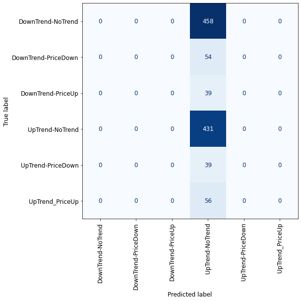
Dummy Classifier
from sklearn.dummy import DummyClassifier

dummy = DummyClassifier()
dummy.fit(X_train, y_train)
pd.DataFrame(cross_validate(dummy, X_train, y_train, return_train_score=True)).mean()
fit_time       0.003735
score_time     0.001221
test_score     0.419318
train_score    0.419317
dtype: float64
plot_confusion_matrix_classifier(dummy) #plotting the confusion matrix for X_test and y_test
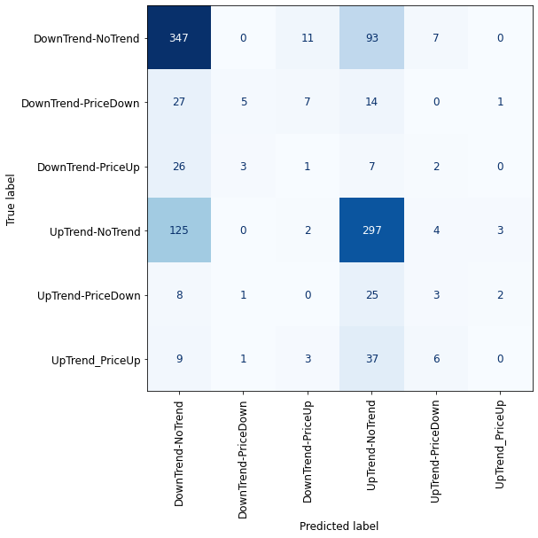
RandomForest
from sklearn.ensemble import RandomForestClassifier

rfc = RandomForestClassifier(max_depth=10, random_state=0)
rfc.fit(X_train, y_train)
pd.DataFrame(cross_validate(rfc, X_train, y_train, return_train_score=True)).mean()
fit_time       1.382421
score_time     0.031423
test_score     0.621547
train_score    0.740597
dtype: float64
plot_confusion_matrix_classifier(rfc) #plotting the confusion matrix for X_test and y_test

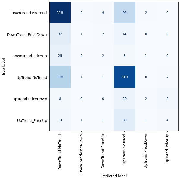
AdaBoost
from sklearn.ensemble import AdaBoostClassifier

adaboost = AdaBoostClassifier(n_estimators=100)
adaboost.fit(X_train, y_train)
pd.DataFrame(cross_validate(adaboost, X_train, y_train, return_train_score=True)).mean()
fit_time       2.602302
score_time     0.058126
test_score     0.573941
train_score    0.594499
dtype: float64
plot_confusion_matrix_classifier(adaboost) #plotting the confusion matrix for X_test and y_test
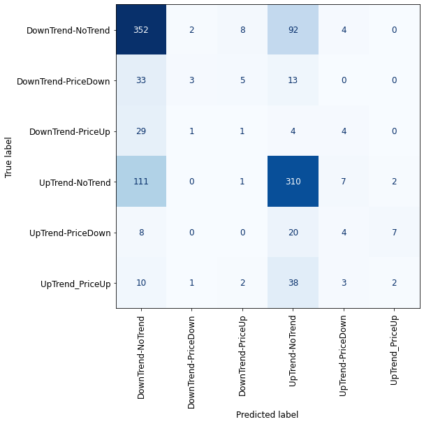
Gradient Boosted Decision Trees
from sklearn.utils import class_weight
from sklearn.ensemble import HistGradientBoostingClassifier

hgbc = HistGradientBoostingClassifier(max_iter=100)
hgbc.fit(X_train, y_train)
pd.DataFrame(cross_validate(hgbc, X_train, y_train, return_train_score=True)).mean()
fit_time       4.151003
score_time     0.069076
test_score     0.601578
train_score    0.973763
dtype: float64
plot_confusion_matrix_classifier(hgbc) #plotting the confusion matrix for X_test and y_test
One-vs-All
from sklearn.multiclass import OneVsRestClassifier

ova_adaboost = OneVsRestClassifier(AdaBoostClassifier(n_estimators=100))
ova_adaboost.fit(X_train, y_train)
pd.DataFrame(cross_validate(ova_adaboost, X_train, y_train, return_train_score=True)).mean()
fit_time       11.210396
score_time      0.216500
test_score      0.624567
train_score     0.665022
dtype: float64
plot_confusion_matrix_classifier(ova_adaboost) #plotting the confusion matrix for X_test and y_test
One-vs-One
from sklearn.multiclass import OneVsOneClassifier

ovo_adaboost = OneVsOneClassifier(AdaBoostClassifier(n_estimators=100))
ovo_adaboost.fit(X_train, y_train)
pd.DataFrame(cross_validate(ovo_adaboost, X_train, y_train, return_train_score=True)).mean()
fit_time       10.252223
score_time      1.013752
test_score      0.616438
train_score     0.676921
dtype: float64
plot_confusion_matrix_classifier(ovo_adaboost) #plotting the confusion matrix for X_test and y_test
Support Vector Machine
from sklearn.svm import SVC

svc = SVC(kernel='rbf', probability=True)
svc.fit(X_train, y_train)
pd.DataFrame(cross_validate(svc, X_train, y_train, return_train_score=True)).mean()
fit_time       4.656176
score_time     0.231267
test_score     0.620849
train_score    0.625493
dtype: float64
plot_confusion_matrix_classifier(svc) #plotting the confusion matrix for X_test and y_test
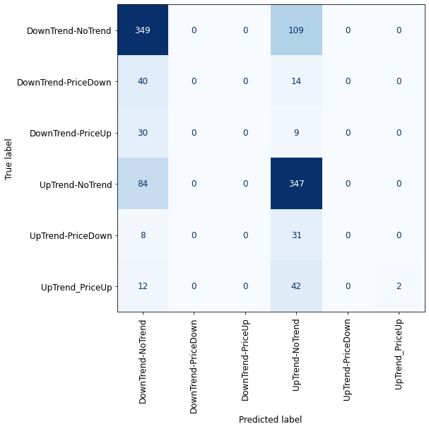
Due to the imbalanced classes, we cannot validate properly the performance of our models, but by looking at the confusion matrixes we can definitely say that all of the classification methods failed here! For sure, having imbalanced classes affected the results, but the nature of the financial market also plays a significant role, especially in the short time frames (5 minutes here) where price has lots of fluctuations.
In the next blog post, I’ll explain how we can deal with the imbalanced classes.